
Mapping Proximity of Dinosaur and Plant Fossils

Zoe Liu
This post is a continuation of my first tutorial where I looked at the dinosaur fossil location data, in this post I will walk through other fossil types in the the Paleobiology Database (PBDB) - plants! We will be exploring how to map different types of fossils onto an interacitve map using plot.ly. We will also look at where and which plant species fossil are most common and introduce a strategy to find which dinosaur fossils are closest to plant fossils to understand the plant landscape and ecosystem in which specific dinosaur species lived (and possibly even ate!).
import pandas as pd
from pathlib import Path
import seaborn as sns
import matplotlib.pyplot as plt

pd.options.mode.chained_assignment = None #ignore Setting with copy warnings
data_file = Path("data/part1", "dino_data.hdf")
interesting = pd.read_hdf(data_file, "interesting")
dino_plants = pd.read_hdf(data_file, "dino_plants")
dino_df = pd.read_hdf(data_file, "dino_df")
Now, let’s take the dinosaur and plant data we gathered above and combine them to see what we can find!
interesting.head() #our cleaned dinosaur data
| accepted_name | state | lat | lng | environment | created | country | early_interval | late_interval | interval | |
|---|---|---|---|---|---|---|---|---|---|---|
| 19 | Theropoda | Connecticut | 41.566666 | -72.633331 | terrestrial indet. | 2011-07-28 02:09:51 | US | Hettangian | Sinemurian | Jurassic |
| 20 | Camarasaurus grandis | Colorado | 39.068802 | -108.699989 | fluvial-lacustrine indet. | 2017-11-02 14:56:21 | US | Kimmeridgian | Tithonian | Jurassic |
| 21 | Camarasaurus supremus | Colorado | 39.111668 | -108.717499 | fluvial-lacustrine indet. | 2001-09-19 09:11:44 | US | Kimmeridgian | NaN | Jurassic |
| 22 | Ankylosaurus magniventris | Montana | 47.637699 | -106.569901 | terrestrial indet. | 2001-09-19 10:03:19 | US | Maastrichtian | NaN | Cretaceous |
| 23 | Titanosauriformes | Oklahoma | 34.180000 | -96.278053 | coastal indet. | 2005-08-25 14:56:00 | US | Late Aptian | Early Albian | Cretaceous |
dino_plants.head() #our cleaned plant data
| accepted_name | state | lat | lng | environment | created | country | early_interval | late_interval | interval | |
|---|---|---|---|---|---|---|---|---|---|---|
| 96 | Neocalamites | New Mexico | 35.200001 | -105.783333 | fluvial indet. | 2001-06-08 06:53:35 | US | Late Triassic | NaN | Triassic |
| 97 | Brachyphyllum | New Mexico | 35.200001 | -105.783333 | fluvial indet. | 2001-06-08 06:53:35 | US | Late Triassic | NaN | Triassic |
| 98 | Masculostrobus | New Mexico | 35.200001 | -105.783333 | fluvial indet. | 2001-06-08 06:53:35 | US | Late Triassic | NaN | Triassic |
| 99 | Samaropsis | New Mexico | 35.200001 | -105.783333 | fluvial indet. | 2001-06-08 06:46:34 | US | Late Triassic | NaN | Triassic |
| 100 | Samaropsis | New Mexico | 35.200001 | -105.783333 | fluvial indet. | 2001-06-08 06:46:34 | US | Late Triassic | NaN | Triassic |
dino_df.head() #our original dinosaur data
| authorizer | authorizer_no | country | collection_no | county | cx_int_no | created | modified | max_ma | reid_no | ... | srb | sro | regional_section | stratscale | state | szn | diference | tec | accepted_no | accepted_name | |
|---|---|---|---|---|---|---|---|---|---|---|---|---|---|---|---|---|---|---|---|---|---|
| 0 | M. Carrano | prs:14 | CA | col:11890 | NaN | 39 | 2011-05-13 07:45:44 | 2011-05-12 16:46:47 | 83.5 | rei:24752 | ... | 4.135 | bottom to top | Dinosaur Park | bed | Alberta | NaN | subjective synonym of | NaN | txn:53194 | Gorgosaurus libratus |
| 1 | M. Carrano | prs:14 | CA | col:11892 | NaN | 39 | 2001-09-18 13:58:56 | 2013-05-10 07:22:24 | 83.5 | NaN | ... | NaN | NaN | NaN | bed | Alberta | NaN | NaN | NaN | txn:38755 | Hadrosauridae |
| 2 | M. Carrano | prs:14 | CA | col:11893 | NaN | 39 | 2010-07-27 08:36:19 | 2010-07-27 10:37:07 | 83.5 | rei:23301 | ... | NaN | NaN | NaN | bed | Alberta | NaN | NaN | NaN | txn:53194 | Gorgosaurus libratus |
| 3 | M. Carrano | prs:14 | CA | col:11894 | NaN | 39 | 2001-09-18 14:04:56 | 2006-04-21 12:43:50 | 83.5 | NaN | ... | 4.03 | NaN | Dinosaur Park | bed | Alberta | NaN | NaN | NaN | txn:63911 | Centrosaurus apertus |
| 4 | M. Carrano | prs:14 | CA | col:11895 | NaN | 39 | 2010-07-27 08:39:37 | 2010-07-27 10:39:58 | 83.5 | rei:23302 | ... | NaN | NaN | NaN | bed | Alberta | NaN | NaN | NaN | txn:53194 | Gorgosaurus libratus |
5 rows × 61 columns
First, we would like to visualize our cleaned and accumulated data. We will use plotly to plot the data points onto a map of the United States.
import plotly
import plotly.plotly as py
import pandas as pd
import plotly.graph_objs as go
from plotly.offline import iplot, init_notebook_mode
from ipywidgets import interactive, HBox, VBox, widgets, interact

plotly.offline.init_notebook_mode()

interesting["text"] = "name: " + interesting["accepted_name"].astype(str)
dinos = {'lat': interesting["lat"],
  'lon': interesting["lng"],
  'marker': {'color': 'rgb(116,0,217)',
   'line': {'color': 'rgb(40,40,40)', 'width': 0.5},
   'size': 2.700000000000003,
   'sizemode': 'diameter'},
  'text': interesting["text"],
  'type': 'scattergeo',
        "name": "Dinosaurs"}

dino_plants["text"] = "name: " + dino_plants["accepted_name"].astype(str)
plants = {'lat': dino_plants["lat"],
  'lon': dino_plants["lng"],
  'marker': {'color': 'rgb(0, 217, 108)',
   'line': {'color': 'rgb(40,40,40)', 'width': 0.5},
   'size': 2.700000000000003,
   'sizemode': 'diameter'},
  'text': dino_plants["text"],
  'type': 'scattergeo',
         "name": "Plants"}

era_range = ["Triassic", "Jurassic", "Cretaceous", "Paleogene", "Neogene", "Quaternary"]

for era in era_range:
    slider_step = {'args': [
            [era]
         ],
         'label': era,
         }

layout = go.Layout(
    title = "Dinosaurs and Plant Fossils of America (Triassic - Quaternary)",
    showlegend = True,
    geo = dict(
            scope='usa',
            projection=dict( type='albers usa'),
            showland = True,
            landcolor = 'rgb(217, 217, 217)',
            subunitwidth=1,
            countrywidth=1,
            subunitcolor="rgb(255, 255, 255)",
            countrycolor="rgb(255, 255, 255)"
        ))
comp_data = [dinos, plants]

fig = go.Figure(layout=layout, data=comp_data)
iplot(fig, validate=False)
Above, we see all the dinosaur and plant fossils found in the United States! We notice a large clustering of data points in Central America. This is due to the fact that much of central US was covered by an inland sea in the Cretaceous era. Rivers covered dinosaur remains with sediment, preserving them as fossils, and the formation of the Rocky Mountains also aided in burying dinosaur remains and fossilizing them.
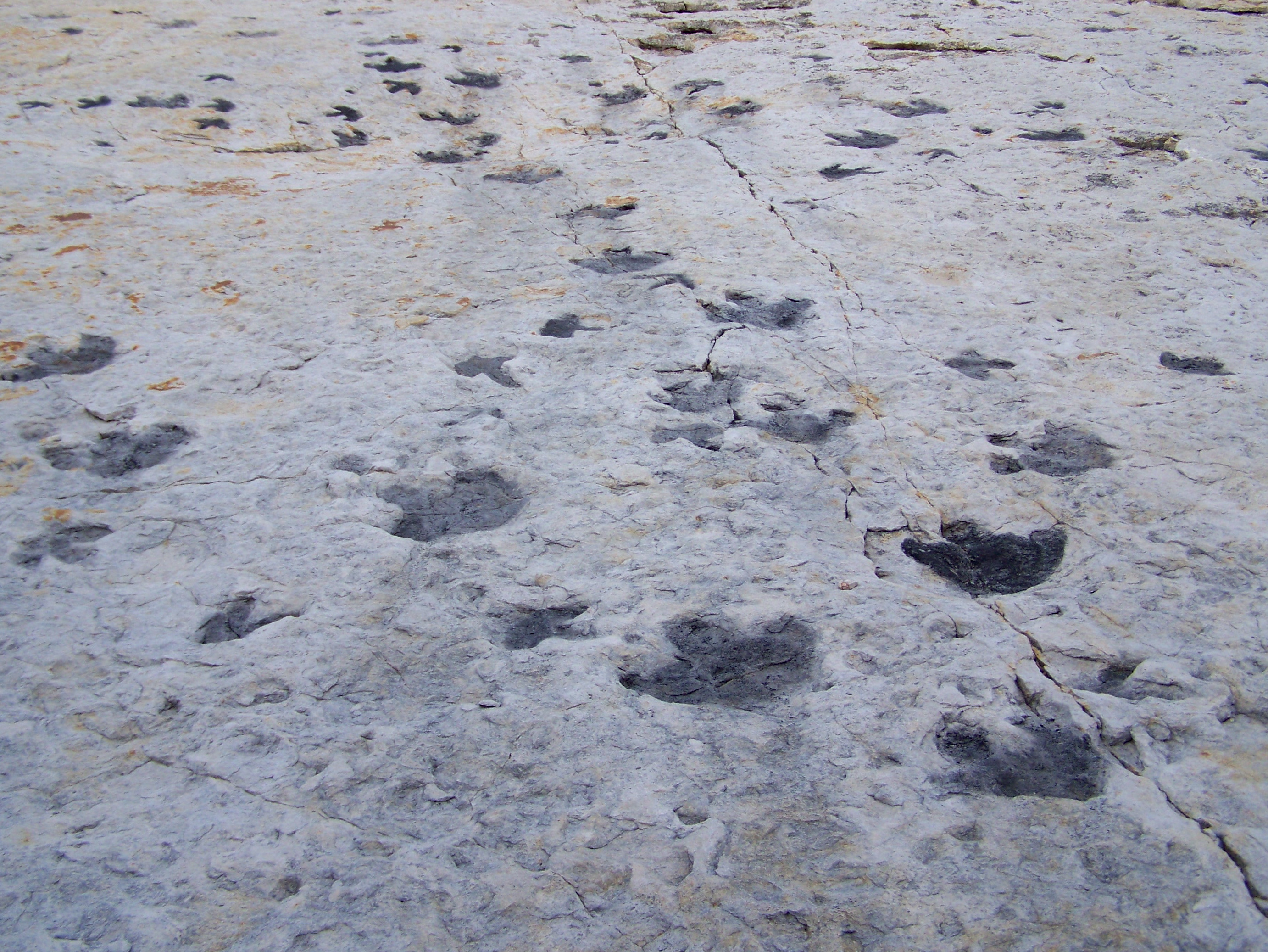
Dinosaur tracks left at Dinosaur Ridge, Colorado, one of the world’s most famous dinosaur fossil sites.
Hadrosaur Diet
From our previous analysis we saw that some of the most prominant dinosaurs in our dataset were Hadrosuars. There is a lot of debate on Hadrosaur diet, it is generally believed that teir diet consisted of vegetation. I thought it would be fun to examine Hadrosaur diet based on plant fossil presence in proximity to Hadrosaurs.
With our newly cleaned data, we can now answer questions we have using our data. For example, what did hadrosaur eat?. Again, this question has been a subject of debate among paleontologists over the past century. From the 1870’s to the 1960’s, it was widely believed that hadrosaurs were only suited to eat soft, aquatic plants. However, later research contended that hadrosaurs only ate land plants such as leaves and twigs. We will attempt to gain further insight on this debate using our data.
First, let’s visualize the spread of hadrosaur fossils. Maybe the location of their fossils can tell us something about what they ate.
interesting["text"] = "name: " + interesting["accepted_name"].astype(str)
hadro = interesting[interesting["accepted_name"] == "Hadrosauridae"]
hadros = {'lat': hadro["lat"],
  'lon': hadro["lng"],
  'marker': {'color': 'rgb(116,0,217)',
   'line': {'color': 'rgb(40,40,40)', 'width': 0.5},
   'size': 2.700000000000003,
   'sizemode': 'diameter'},
  'text': hadro["text"],
  'type': 'scattergeo',
        "name": "Dinosaurs"}

dino_plants["text"] = "name: " + dino_plants["accepted_name"].astype(str)
nm = dino_plants[dino_plants["state"] == "New Mexico"]
plants = {'lat': nm["lat"],
  'lon': nm["lng"],
  'marker': {'color': 'rgb(0, 217, 108)',
   'line': {'color': 'rgb(40,40,40)', 'width': 0.5},
   'size': 2.700000000000003,
   'sizemode': 'diameter'},
  'text': nm["text"],
  'type': 'scattergeo',
         "name": "Plants"}


layout = go.Layout(
    title = "Hadrosauridae Fossils of America (Triassic - Quaternary)",
    showlegend = True,
    geo = dict(
            scope='usa',
            projection=dict( type='albers usa'),
            showland = True,
            landcolor = 'rgb(217, 217, 217)',
            subunitwidth=1,
            countrywidth=1,
            subunitcolor="rgb(255, 255, 255)",
            countrycolor="rgb(255, 255, 255)"
        ))

fig = go.Figure(layout=layout, data=[hadros])
iplot(fig, validate=False)
We notice that the majority of the hadrosaurs are located in Central North America. While we don’t know exactly the river and lakes that could have exsisted in this area during this time. We can rule out that hadrosaurs ate oceann aquatic plants due to the location of the fossils in landlocked areas.
Let’s examine the relationship between hadrosaur fossil coordinates and plant fossil coordinates. We’ll take the coordinates of the hadrosaur and plant fossils, zip them into a list, and add them to our dataframe. But first, let’s remove all instances of “Plantae” from our dino_plant dataframe, since Plantae is a broad generalization of any plant and isn’t very useful.
dino_plants = dino_plants[dino_plants["accepted_name"] != "Plantae"]
hadro["coords"] = list(zip(hadro.lat, hadro.lng))
dino_plants["coords"] = list(zip(dino_plants.lat, dino_plants.lng))
hadro.head()
| accepted_name | state | lat | lng | environment | created | country | early_interval | late_interval | interval | text | coords | nearest_plant | |
|---|---|---|---|---|---|---|---|---|---|---|---|---|---|
| 26 | Hadrosauridae | Montana | 47.695831 | -106.227776 | "channel" | 2002-01-15 15:16:43 | US | Maastrichtian | NaN | Cretaceous | name: Hadrosauridae | (47.695831, -106.227776) | Plantae |
| 63 | Hadrosauridae | Wyoming | 43.349400 | -104.482002 | "channel" | 2002-07-10 20:49:32 | US | Maastrichtian | NaN | Cretaceous | name: Hadrosauridae | (43.3494, -104.482002) | Celastrus |
| 118 | Hadrosauridae | Texas | 29.138056 | -103.196945 | fine channel fill | 2002-07-10 20:49:32 | US | Late Campanian | NaN | Cretaceous | name: Hadrosauridae | (29.138056, -103.196945) | Selaginella |
| 147 | Hadrosauridae | Montana | 48.966599 | -112.650002 | lacustrine - small | 2002-07-10 20:49:32 | US | Campanian | NaN | Cretaceous | name: Hadrosauridae | (48.966599, -112.650002) | Protophyllum |
| 186 | Hadrosauridae | New Jersey | 40.299999 | -74.300003 | estuary/bay | 2002-08-20 14:43:52 | US | Judithian | NaN | Cretaceous | name: Hadrosauridae | (40.299999, -74.300003) | Microaltingia apocarpela |
hadro["interval"].value_counts()
Cretaceous    460
Name: interval, dtype: int64
hadro["interval"].value_counts().index[0]
'Cretaceous'
Because the hadrosaurs were only found in the Cretaceous era, we can filter our dino_plant dataframe to only contain plants in the Cretaceous era.
cret_plants = dino_plants[dino_plants["interval"] == "Cretaceous"]
cret_plants.head()
| accepted_name | state | lat | lng | environment | created | country | early_interval | late_interval | interval | text | coords | |
|---|---|---|---|---|---|---|---|---|---|---|---|---|
| 3175 | Ginkgo | Arizona | 31.811390 | -110.418053 | fluvial indet. | 2002-01-21 11:54:06 | US | Late Albian | Early Cenomanian | Cretaceous | name: Ginkgo | (31.81139, -110.418053) |
| 3176 | Cycadophyta | Arizona | 31.811390 | -110.418053 | fluvial indet. | 2002-01-21 11:54:06 | US | Late Albian | Early Cenomanian | Cretaceous | name: Cycadophyta | (31.81139, -110.418053) |
| 3579 | Magnoliid | Nebraska | 40.056946 | -97.182777 | fluvial indet. | 2002-06-07 13:31:38 | US | Early Cenomanian | Middle Cenomanian | Cretaceous | name: Magnoliid | (40.056946, -97.182777) |
| 3580 | Pandemophyllum | Nebraska | 40.056946 | -97.182777 | fluvial indet. | 2002-06-07 13:59:40 | US | Early Cenomanian | Middle Cenomanian | Cretaceous | name: Pandemophyllum | (40.056946, -97.182777) |
2776 rows × 12 columns
Next, we’ll use the KDTree, or a k-dimensional tree, data structure to find the nearest plant neighbor to each hadrosaurus fossil. Then, we’ll extract the accepted name of each plant and add it to our DataFrame for examination.
from scipy import spatial
closest = []
all_plants = cret_plants["coords"].values.tolist()
tree = spatial.KDTree(all_plants)
for coord in hadro["coords"]:
    query = tree.query([coord])
    closest += [query]
import numpy as np
hadro_plant = []
for i in np.arange(len(closest)):
    index = closest[i][1][0]
    hadro_plant += [cret_plants.iloc[index]["accepted_name"]]
hadro["nearest_plant"] = hadro_plant
hadro.head()
| accepted_name | state | lat | lng | environment | created | country | early_interval | late_interval | interval | text | coords | nearest_plant | |
|---|---|---|---|---|---|---|---|---|---|---|---|---|---|
| 26 | Hadrosauridae | Montana | 47.695831 | -106.227776 | "channel" | 2002-01-15 15:16:43 | US | Maastrichtian | NaN | Cretaceous | name: Hadrosauridae | (47.695831, -106.227776) | Azolla |
| 63 | Hadrosauridae | Wyoming | 43.349400 | -104.482002 | "channel" | 2002-07-10 20:49:32 | US | Maastrichtian | NaN | Cretaceous | name: Hadrosauridae | (43.3494, -104.482002) | Celastrus |
| 118 | Hadrosauridae | Texas | 29.138056 | -103.196945 | fine channel fill | 2002-07-10 20:49:32 | US | Late Campanian | NaN | Cretaceous | name: Hadrosauridae | (29.138056, -103.196945) | Selaginella |
| 147 | Hadrosauridae | Montana | 48.966599 | -112.650002 | lacustrine - small | 2002-07-10 20:49:32 | US | Campanian | NaN | Cretaceous | name: Hadrosauridae | (48.966599, -112.650002) | Protophyllum |
| 186 | Hadrosauridae | New Jersey | 40.299999 | -74.300003 | estuary/bay | 2002-08-20 14:43:52 | US | Judithian | NaN | Cretaceous | name: Hadrosauridae | (40.299999, -74.300003) | Microaltingia apocarpela |
460 rows × 13 columns
Now let’s visually examine the nearest plant to hadrosaurs.
plt.figure(figsize=(12,6)) #create a figure that is 12 x 6
ax = sns.countplot(x='nearest_plant', data=hadro, order=hadro['nearest_plant'].value_counts().index.tolist()[:20])
ax.set_xticklabels(ax.get_xticklabels(), rotation=90)
plt.title("Top 20 Nearest Plant to Hadrosauridae (Except Plantae)")
plt.show()
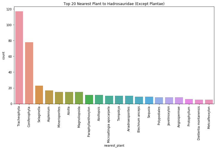
Our most common plant is of the clade tracheophyta, or vascular plants, which is a broad umbrella term for a number of land plants with xylems that conduct water throughout the plant body. Second on our list is coniferophyta, or cone-bearing trees like pines, cypresses, and spruces. This is phylogenetically a descendant of the tracheophyta, and it is plausible that some of the tracheophyta fossils found are potentially conifers. This abundance of land plants near the hadrosaur fossils supports the idea that hadrosaurs ate land plants like conifer needles and fruit. As a matter of fact, John Ostrom, a revolutionary paleontologist, showed in 1964 that there was little evidence of hadrosaurs having an aquatic diet. For one, aquatic plant pollen was very uncommon near the hadrosaur herds he was investigating (as we can see from our data above). This argument was further supported by a 1922 study of the gut contents of hadrosaurs, which found conifer needles, fruit, and seeds.

An example of a tracheophyte. Note the feathery fronds of the plant, which are vascular tissues that carry water throughout the plant.
Again, this is a very superficial way to explore Dinosaur diet, but let’s look into plant proximity to dinosaurs a bit broader. Now that we’ve explored what the hadrosaurs might have eaten based on the nearest fossilized plants, let’s expand this to all other dinosaurs. What did every type of dinosaurs eat based on proximity?
To answer this question, we have to know:
- The coordinates of every dinosaur, grouped by type
- The coordinates of every plant fossil originating from the same geologic period
Using KDTrees to find proximity of latitude and longitude points
KDtrees are a way to organize points in space and a very useful strategy for finding nearest neighbor searches. We can construct a KDTree and find the nearest plant fossil to each dinosaur. To make this easier, we can construct six KDTrees, each corresponding to a different geologic period, and run them on the dinosaurs in the same period.
First, let’s create a function that will filter out plant fossils by geologic period. This will aid us in creating the period-grouped KDTrees.
def make_period_plant(period):
    period_plants = dino_plants[dino_plants["interval"] == period]
    return period_plants
cret_plants = make_period_plant("Cretaceous")
jur_plants = make_period_plant("Jurassic")
tri_plants = make_period_plant("Triassic")
neo_plants = make_period_plant("Neogene")
paleo_plants = make_period_plant("Paleogene")
quat_plants = make_period_plant("Quaternary")
Next, we’ll construct a KDTree for each geologic period. Below, I’ve grouped the dinosaur dataframe interesting by interval, which will make it easier to iterate through every item in each group and apply every dinosaur data point to the constructed KDTree. At the end, we end up with six dataframes, with rows corresponding to each dinosaur fossil and their nearest plant fossil. We merge these together and our resulting dataframe, dinonplants, is the same as interesting, except with a nearest_plant column.
dinonplants = pd.DataFrame()
grouped = interesting.groupby("interval")
for interval, groups in grouped:
    if interval == "Cretaceous":
        plants = cret_plants
    elif interval == "Jurassic":
        plants = jur_plants
    elif interval == "Triassic":
        plants = tri_plants
    elif interval == "Neogene":
        plants = neo_plants
    elif interval == "Paleogene":
        plants = paleo_plants
    elif interval == "Quaternary":
        plants = quat_plants

    print("Calculating: ", interval)
    values = grouped.groups.get(interval)
    new_df = interesting[interesting.index.isin(values)]

    new_df["coords"] = list(zip(new_df.lat, new_df.lng))
    plants["coords"] = list(zip(plants.lat, plants.lng))
    closest = []
    all_plants = plants["coords"].values.tolist()
    tree = spatial.KDTree(all_plants)
    for coord in new_df["coords"]:
        query = tree.query([coord], k=2)
        closest += [query[1][0][0]] #list of nearest plant indices
    nearest_plant = []
    for i in closest:
        nearest_plant += [plants.iloc[i]["accepted_name"]]
    new_df["nearest_plant"] = nearest_plant
    dinonplants = dinonplants.append(new_df, ignore_index=False)
Calculating:  Cretaceous
Calculating:  Jurassic
Calculating:  Neogene
Calculating:  Paleogene
Calculating:  Quaternary
Calculating:  Triassic
dinonplants = dinonplants.sort_index() #this sorts the merged dataframe by increasing index
dinonplants.head()
| accepted_name | state | lat | lng | environment | created | country | early_interval | late_interval | interval | text | coords | nearest_plant | |
|---|---|---|---|---|---|---|---|---|---|---|---|---|---|
| 19 | Theropoda | Connecticut | 41.566666 | -72.633331 | terrestrial indet. | 2011-07-28 02:09:51 | US | Hettangian | Sinemurian | Jurassic | name: Theropoda | (41.566666, -72.633331) | Baiera |
| 20 | Camarasaurus grandis | Colorado | 39.068802 | -108.699989 | fluvial-lacustrine indet. | 2017-11-02 14:56:21 | US | Kimmeridgian | Tithonian | Jurassic | name: Camarasaurus grandis | (39.068802, -108.699989) | Tracheophyta |
| 21 | Camarasaurus supremus | Colorado | 39.111668 | -108.717499 | fluvial-lacustrine indet. | 2001-09-19 09:11:44 | US | Kimmeridgian | NaN | Jurassic | name: Camarasaurus supremus | (39.111668, -108.717499) | Tracheophyta |
| 22 | Ankylosaurus magniventris | Montana | 47.637699 | -106.569901 | terrestrial indet. | 2001-09-19 10:03:19 | US | Maastrichtian | NaN | Cretaceous | name: Ankylosaurus magniventris | (47.637699, -106.569901) | Azolla |
| 23 | Titanosauriformes | Oklahoma | 34.180000 | -96.278053 | coastal indet. | 2005-08-25 14:56:00 | US | Late Aptian | Early Albian | Cretaceous | name: Titanosauriformes | (34.18, -96.278053) | Dichastopollenites |
9143 rows × 13 columns
Now that we’ve obtained the nearest plant to every individual fossil, let’s group these fossils by name and pick out the highest occurring nearest plant. What we end up with is a table that shows every type of dinosaur fossil and their most frequently seen nearest plant.
vals = dinonplants.groupby("accepted_name")["nearest_plant"].agg(lambda x:x.value_counts().index[0])
dinos_nearest_plant = vals.to_frame()
dinos_nearest_plant.head()
| nearest_plant | |
|---|---|
| accepted_name | |
| Abydosaurus mcintoshi | Magnoliopsida |
| Accipiter cooperii | Vitis |
| Accipiter gentilis | Pinus |
| Accipiter striatus | Carya |
| Accipiter striatus velox | Zosteraceae |
As a sanity check, let’s make sure that the nearest plant to Hadrosauridae is the Tracheophyta (which we found in our exercise on hadrosaur diet above).
dinos_nearest_plant.loc["Hadrosauridae"]
nearest_plant    Tracheophyta
Name: Hadrosauridae, dtype: object
Great, our code looks correct. Now let’s perform some visual analysis on the data we collected. What plants were every type of dinosaur eating the most?
plt.figure(figsize=(12,6)) #create a figure that is 12 x 6
ax = sns.countplot(x='nearest_plant', data=dinonplants, order=dinonplants['nearest_plant'].value_counts().index.tolist()[:20])
ax.set_xticklabels(ax.get_xticklabels(), rotation=90)
plt.title("Nearest Plant (Except Plantae) to Each Type of Dinosaur")
plt.show()
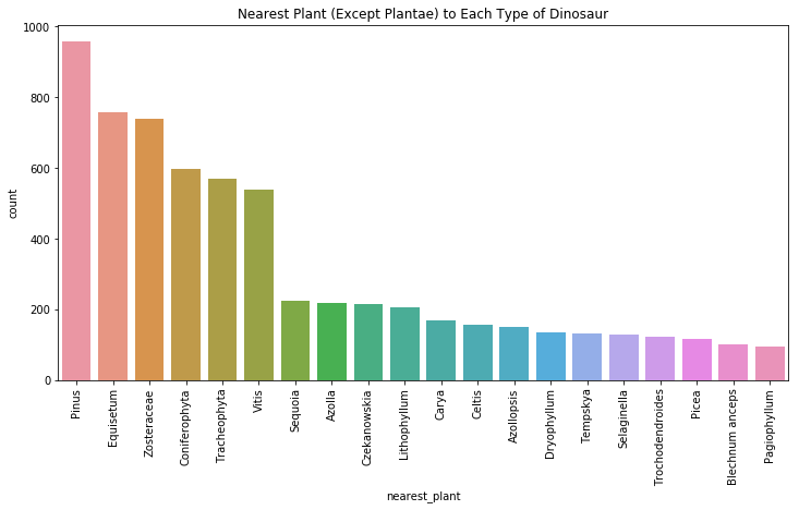
Pinus, or pine trees, equisetum, or horsetail grass, and zosteraceae, a type of seagrass, are the most commonly found plants. These findings aren’t too surprising. Paleontologists have known for decades that herbivorous dinosaurs fed on plants like pine needles, evergreen conifers (such as redwoods, and pine trees), horsetail grass, and seagrasses.

Horsetail grass, or equisetum, are considered living fossils due to the fact that they haven’t changed in the past 100 million years. In the age of the dinosaurs, they could grow up to 30 meters tall, though they typically only grow 1 m tall in the modern age.
Now let’s visualize some period-specific dinosaur and plant relations.
period_plants = dinonplants.groupby(["accepted_name", "interval"])["nearest_plant"].agg(lambda x:x.value_counts().index[0])
period_plant_df = period_plants.to_frame()
period_plant_df.head()
| nearest_plant | ||
|---|---|---|
| accepted_name | interval | |
| Abydosaurus mcintoshi | Cretaceous | Magnoliopsida |
| Accipiter cooperii | Quaternary | Vitis |
| Accipiter gentilis | Quaternary | Pinus |
| Accipiter striatus | Quaternary | Carya |
| Accipiter striatus velox | Quaternary | Zosteraceae |
cret_dinonplants = period_plant_df[period_plant_df.index.get_level_values(1) == "Cretaceous"]
plt.figure(figsize=(12,6)) #create a figure that is 12 x 6
ax = sns.countplot(x='nearest_plant', data=cret_dinonplants, order=cret_dinonplants['nearest_plant'].value_counts().index.tolist()[:20])
ax.set_xticklabels(ax.get_xticklabels(), rotation=90)
plt.title("Nearest Plant (Except Plantae) to Each Type of Dinosaurs in Cretaceous Era")
plt.show()
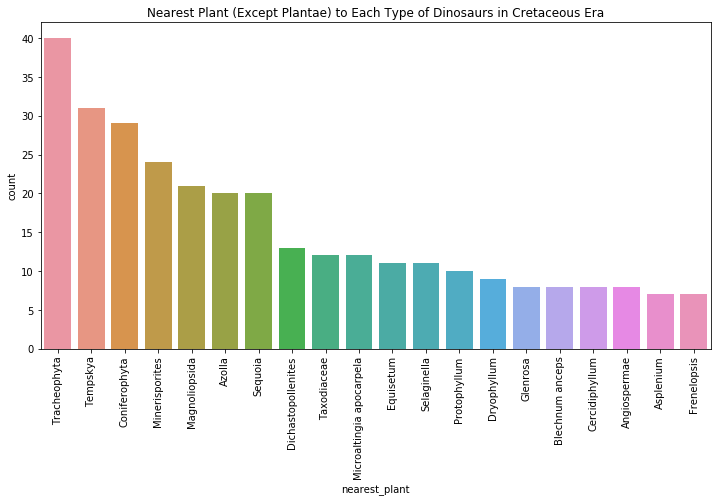
This graph shows much of the same trends as the chart showing plants closest to hadrosaurs, which makes sense, as hadrosaurs were common in the Cretaceous period.
quat = period_plant_df[period_plant_df.index.get_level_values(1) == "Quaternary"]
plt.figure(figsize=(12,6)) #create a figure that is 12 x 6
ax = sns.countplot(x='nearest_plant', data=quat, order=quat['nearest_plant'].value_counts().index.tolist()[:20])
ax.set_xticklabels(ax.get_xticklabels(), rotation=90)
plt.title("Nearest Plant (Except Plantae) to Each Type of Dinosaurs in Quaternary Period")
plt.show()
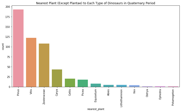
In the Quaternary period, we start moving into familiar territory. The dinosaurs in this period (which have now evolved to be the birds we know today) were around common plants like pine trees (pinus) and grape vines (vitis).
In Conclusion
In this section, we visualized our plant and dinsoaur data by plotting them onto a map. We were able to visually comprehend the spatial relationship between plant and dinosaur fossils, and saw that central USA was a popular dinosaur graveyard. With our cleaned data, we were able to answer questions like “what did hadrosaur eat?” by performing a nearest neighbor search of every hadrosaur fossil on plant fossils in the same geologic period. We saw that hadrosaurs were likely feeding on conifers due to the abundance of conferophyta and land plant fossils. We were able to scale up our question by looking at the likely diets of every other type of dinosaur. We ran six different KDTrees, corresponding to the geologic periods, and found the nearest plant fossil to every dinosaur fossil in each. By looking at the most common nearest plant to every dinosaur fossil, we were able to make a guess that the dinosaur in question was feeding on that plant. Some things to keep in mind:
- Our analysis did not account for carnivorous dinosaurs, since we assumed all dinosaurs eat plants. Our question can be rephrased to “what is the spatial relationship between dinosaur fossils and plant fossils?” instead, if we cared about this difference.
- Visualization is a fantastic way of guiding research questions. Think back to how we second guessed the hadrosaur diet of sea plants based on the spread of hadrosaur fossils in land-locked areas. Visualizations can be just as important as more math-based methods when it comes to analytics.
Thank you for reading, and I hope this tutorial has clarified the methods of exploratory analysis, data cleaning, and data analysis.